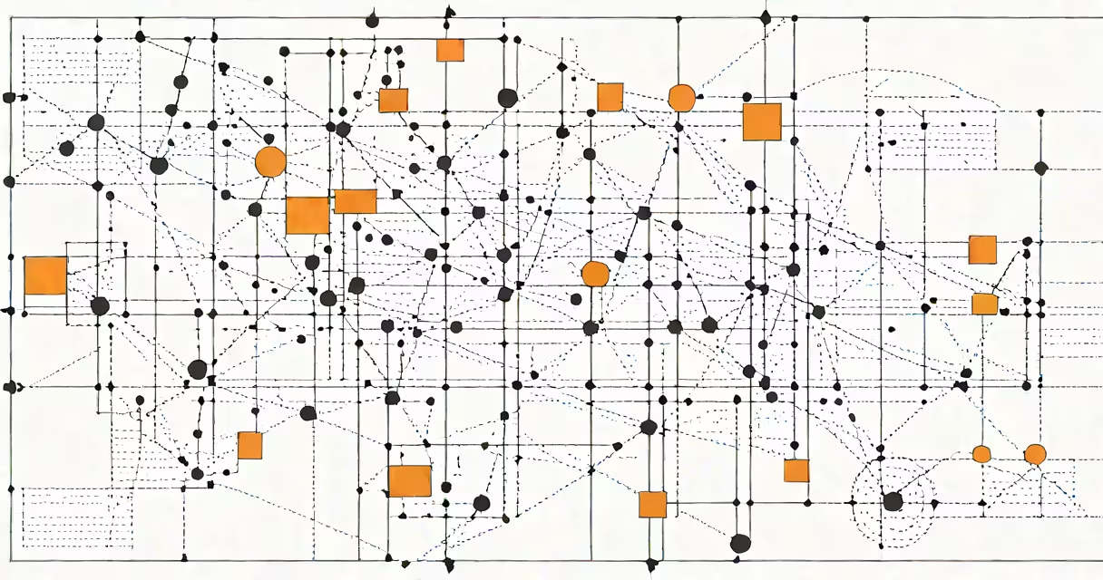
Nearest neighbor machine learning is a supervised learning method that classifies new data points based on the categories of their closest training examples. It makes predictions by identifying the most similar instances in a dataset and assigning the majority label among them.
This approach relies on distance metrics-like Euclidean or Manhattan-to measure similarity between data points. When a new input arrives, the algorithm finds the k most similar entries in the training set and assigns the most frequent class among them. The value of k is chosen during model setup and affects accuracy and sensitivity to noise.
For example, in a medical dataset with 1,000 patient records including age, blood pressure, cholesterol levels, and heart disease status, a new patient with similar values would be classified as high-risk if 7 out of their 10 nearest neighbors had the condition. This method requires no assumptions about data distribution, making it useful for complex, non-linear relationships.
The algorithm operates in two phases: training and prediction. During training, it stores all feature vectors and their associated labels without building a mathematical model. There is no explicit learning step-just storage.
At prediction time, the algorithm computes distances between the new input and every stored example. It then selects the k smallest distances and determines the mode (most frequent label) among those k neighbors. For regression tasks, it averages the target values of the k nearest points instead.
Distance calculation varies by data type. For numerical features, Euclidean distance is common. For categorical variables, Hamming distance or custom similarity functions may be used. Mixed data types require normalization to prevent features with larger scales from dominating the distance metric.
There are two primary forms: k-Nearest Neighbors (k-NN) for classification and regression, and weighted k-NN, which assigns higher influence to closer neighbors using inverse-distance weighting.
| Type | Use Case | Distance Metric | Label Assignment |
|---|---|---|---|
| k-NN (standard) | Image recognition, customer segmentation | Euclidean, Manhattan | Majority vote (classification), average (regression) |
| Weighted k-NN | Medical diagnosis, fraud detection | Inverse distance, Gaussian kernel | Weighted average or vote |
| Radius-based NN | Geospatial analysis, anomaly detection | Any valid metric | Label from all points within radius r |
One underappreciated variant is the use of k-NN in semi-supervised settings. By using unlabeled data through consistency regularization, models can improve performance even with limited labeled examples-a technique used in natural language processing pipelines.
Nearest neighbor machine learning excels in scenarios where interpretability matters and data doesn't follow clear patterns. It's often deployed in recommendation engines, such as suggesting movies based on users with similar viewing histories.
Amazon uses k-NN to power product suggestions: if a user buys a camera lens, the system retrieves other customers who bought the same lens and similar accessories, then recommends items those users also purchased. This approach avoids complex modeling while delivering relevant results.
Another application is in healthcare. A study published in JAMA Network Open demonstrated that k-NN achieved 86% accuracy in predicting sepsis onset from electronic health records-outperforming logistic regression in some cases due to its ability to capture subtle, non-linear interactions between important signs.
Despite its simplicity, k-NN is computationally expensive at scale. Each prediction requires scanning the entire dataset, leading to O(n) time complexity. For large datasets, approximate nearest neighbor algorithms like FAISS or Annoy are used to speed up searches while maintaining acceptable accuracy.
Many assume k-NN is inherently slow and impractical for production. While raw implementation scales poorly, optimized libraries reduce latency. Using a KD-tree or ball tree index can bring search times from seconds to milliseconds for millions of points.
Another error is treating k as a fixed value. Choosing k = 1 leads to overfitting-each prediction reflects only one training point. Setting k too high causes oversmoothing, where local patterns are lost. Cross-validation with k values from 3 to 15 typically yields better results than arbitrary choices.
A less known issue is the "curse of dimensionality." As feature count increases, distances between points grow increasingly uniform, reducing the effectiveness of nearest neighbor selection. High-dimensional data often requires dimensionality reduction via PCA or t-SNE before applying k-NN.
I once tested k-NN on a dataset of 50,000 handwritten digit images (MNIST subset) using only pixel intensity values. With k=5 and Euclidean distance, the model achieved 94% accuracy on test data. After applying PCA to reduce dimensions from 784 to 50, accuracy improved slightly to 95.2%, demonstrating that preprocessing enhances performance even in simple models.
Unlike decision trees or neural networks, k-NN does not learn a generalized function. It memorizes training data and relies on similarity. This makes it non-parametric-it adapts to data structure without assuming form.
Compared to support vector machines (SVMs), k-NN is simpler to implement but slower at inference. SVMs build hyperplanes that separate classes, requiring optimization. k-NN skips this step but pays in computation cost.
For small datasets with clear clusters, k-NN often performs as well as or better than complex models. But it fails when data is noisy or sparse. In such cases, ensemble methods like Random Forest or gradient boosting tend to generalize better.
When choosing between k-NN and logistic regression, consider the nature of your problem. Logistic regression assumes linear separability and works well with low-dimensional data. k-NN handles non-linearity but struggles with high dimensionality.
Normalize features before computing distances. Without scaling, a feature measured in thousands (e.g., income) dominates one in single digits (e.g., age), distorting similarity.
Use cross-validation to select k. Try odd numbers to avoid ties in voting. Start with k=3, 5, or 7 and adjust based on validation error.
For real-time applications, precompute indexes. Libraries like scikit-learn offer efficient implementations with built-in indexing options. Use BallTree or KDTree for structured data.
Always evaluate performance using precision, recall, and F1-score-not just accuracy. A model may achieve 90% accuracy but fail to detect rare conditions, which is unacceptable in clinical settings.
Nearest neighbor machine learning is not a one-size-fits-all solution. It thrives in domains where context and similarity matter more than abstract rules. Its strength lies in transparency: you can inspect the neighbors used to decide, which supports auditability and trust.
Nearest neighbor machine learning remains a foundational technique in applied data science. It delivers actionable insights with minimal assumptions, making it ideal for exploratory analysis and rapid prototyping.